Percolation Exercises

Background
Percolation theory is the study of the connectivity of networks. If you
take a piece of paper and punch small holes in it at random positions, it
will remain connected if the density of holes is small. If you punch so
many holes that most of the paper has been punched away, the paper will
fall apart into small clusters.
There is a phase transition in percolation, where the paper first
falls apart. Let p be the probability that a given spot in the
paper has been punched away. There is a critical probability
pc below which the paper is still connected from top to
bottom, and above which the paper has fallen into small pieces (say, if it
is being held along the top edge).
Learning Goals
Science: You will learn about percolation transitions on
networks, and of universality of critical phenomena near the
percolation critical point.
Computation:
You will first use breadth-first search techniques to compute the set
of connected components (clusters) in an undirected graph.
Then the scaling exercise introduces scaling and critical phenomena methods
for studying the phase transtion for percolation.
Procedure
By now, you should have completed the
Introduction to Networks exercise, and should have working code to
create undirected graphs. If you've already done the
Small world networks exercise (this
is not a prerequisite), then the concept of breadth-first searches
should be clear to you.
Creating bond percolation networks
- Consult the material in Percolation Computation Exercise
for an overview of the exercise and details on writing algorithms.
- Download the file
PercolationHints.py
from the course webpage,
and save it as "Percolation.py". It is easiest if you store this file
in the same directory as the networks files you worked with earlier
(Networks.py and NetGraphics.py), since those files will be needed for
this exercise. [If you need those files, you can get them from the following links Answers file for network
algorithms and
Network graphics software -- be careful not to overwrite the files you previously
made, it would be a shame to loose all that hard work.]
- Build a bond percolation network on a 2D square lattice with
periodic boundary conditions.
Define a function MakeSquareBondPercolation that takes two
arguments, the size of the lattice in each dimension (L), and the
probability that any given bond between nearest neighbors exists (p).
(As with ring graphs, the easiest way to implement periodic boundary
conditions is to use the Python
modular arithmetic operator %:
see the
python documentation.)
This routine will create an instance of the
UndirectedGraph class defined in the
Introduction to Networks exercise.
Finding connected components in networks
- You will now write functions for finding clusters (connected components)
in undirected graphs. This will involve writing and debugging the
following routines: FindClusterFromNode and FindAllClusters.
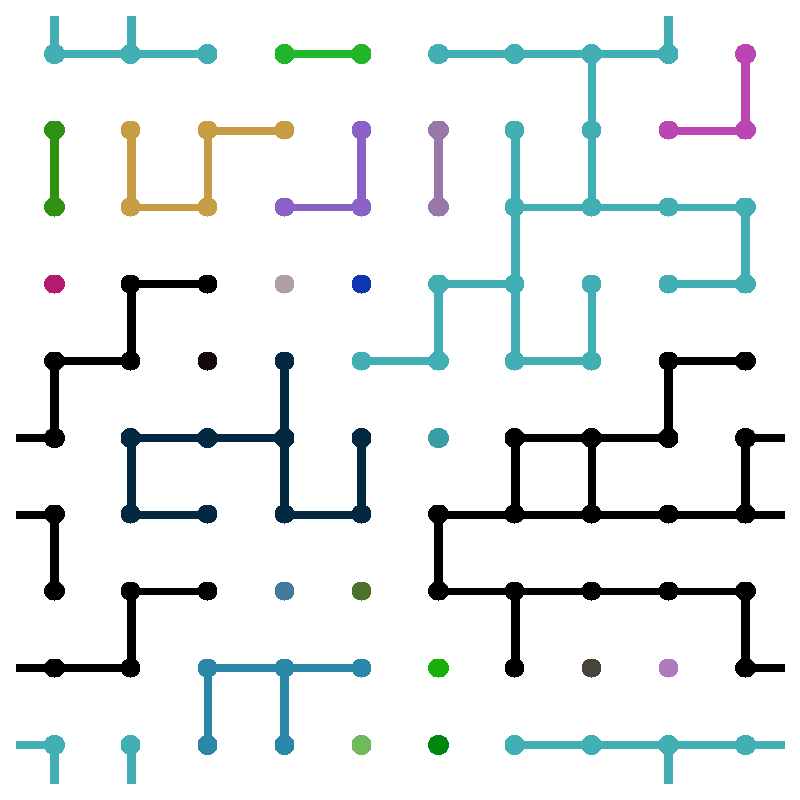
- Use the graphics software provided in NetGraphics.DrawSquareNetworkBonds to visualize the different clusters in the percolation network.
Creating site percolation networks
In bond percolation, bonds are created (or cut) at random. In site
percolation, sites are occupied (or removed) at random, and bonds in
the corresponding graph are inferred if two neighboring sites are
occupied. The same UndirectedGraph class can be used in both
cases, just with different algorithms for populating such graphs.
- Build a site percolation network on a 2D triangular lattice with
periodic boundary conditions.
Define a function MakeTriangularSitePercolation that takes two
arguments, the size of the lattice in each dimension (L), and the
probability that any given site is occupied (p).
- Test your cluster finding function on the site percolation lattice.
(It should work with no modifications if you've written it correctly.)
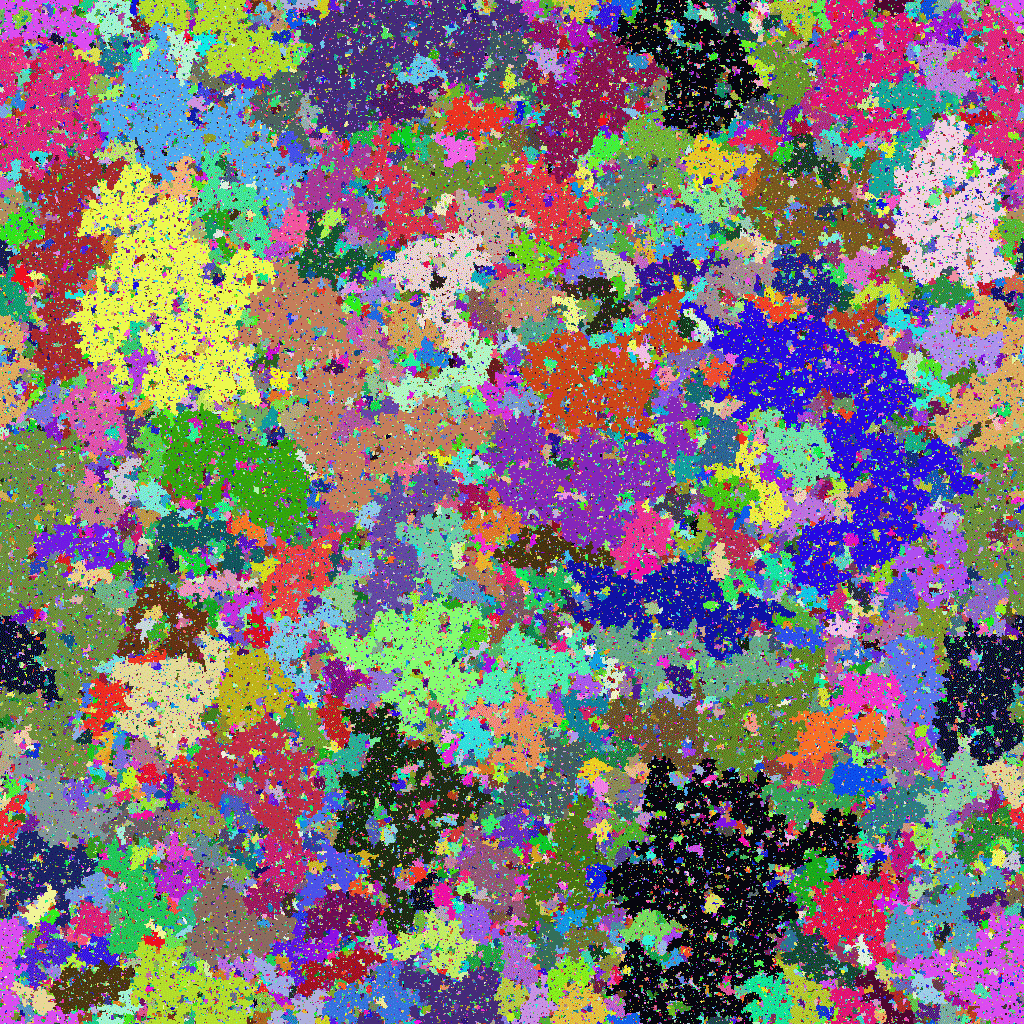
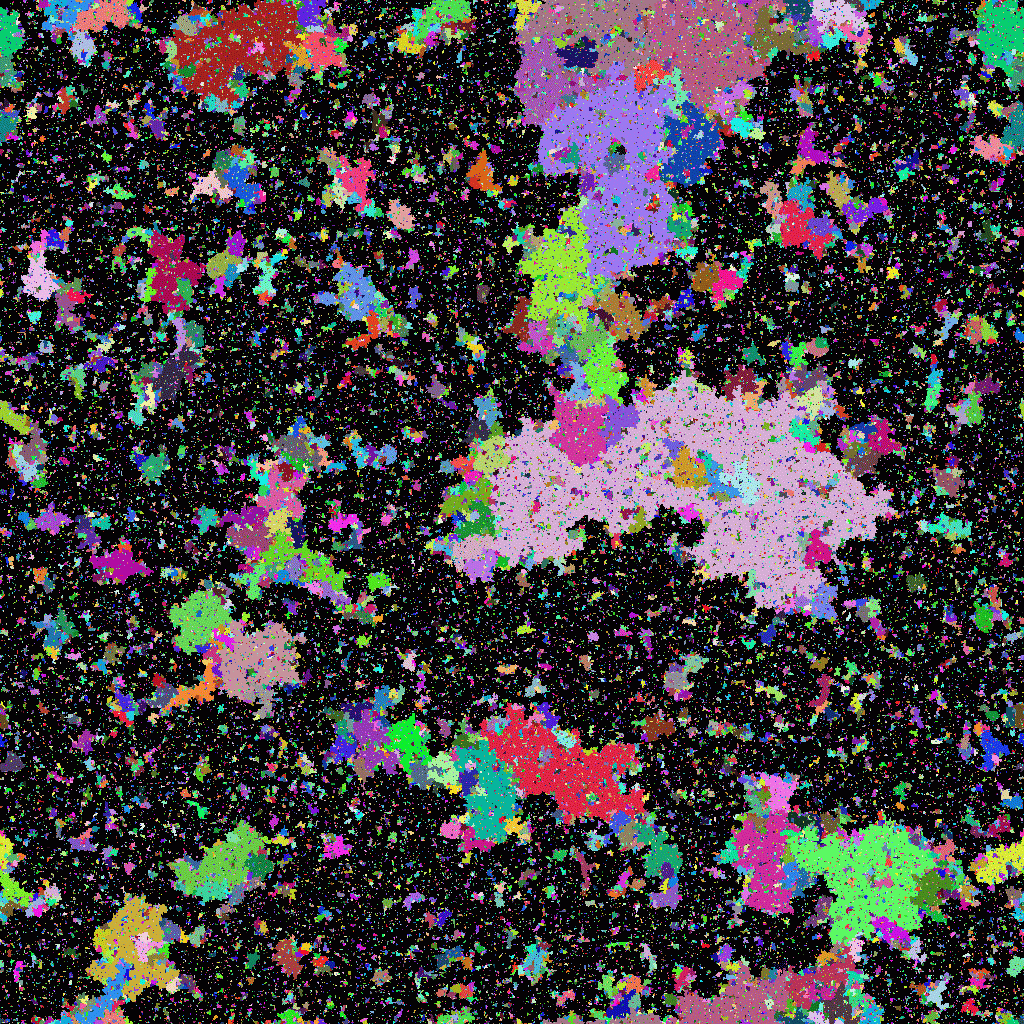
- Use the graphics software provided in NetGraphics.DrawTriangularNetworkSites to visualize the different clusters in the percolation network.
Scaling analyses of percolation networks
- Consult the material in Percolation Scaling Exercise
(Exercise 12.12)
for an overview of the critical phenomena of percolation, the use
of scaling theory to understand such phenomena, and specifics of
computations to be performed.
- (Exercise 12.12(b))
For both bond percolation on the square lattice and site percolation on
the triangular lattice, calculate the cluster size distribution n(S) for
L=400 and p=p_c=0.5. Plot log(n(S)) versus log(S) for both, along
with the theoretical result n(S) ~ S^(-187/91). Do the data show
evidence of power-law cluster size distributions?
- (Exercise 12.12(c))
For both bond percolation on the square lattice and site percolation on
the triangular lattice, calculate the fraction of nodes that are part of
the largest cluster, for L=400 and p=p_c+2^(-n) for n from roughly 0 to 9.
Plot log(P(p)) versus p-p_c, and compare with the theoretical prediction
P(p) ~ (p_c-p)^(5/36).
- (Exercise 12.12(d,e,f,g))
Explore finite size scaling in bond and site percolation, using
scaling collapses to relate simulation data for different system
size L and bond/site fraction p.
Useful Constructions/Syntax
Files
References
Links
Notes
When you try to import a module in Python (e.g., via import somemodule), the interpreter looks through a sequence of directories to find the
specified module. This sequence (a Python list) is stored in the variable
sys.path: you can see what is in the default search path by
first importing the sys module (import sys) and then printing
the path (print sys.path). You will see that an empty directory
('') is in the path; this corresponds to your current directory.
For this reason, it is often easiest to put a group of related files together
in the same directory, such as is recommended here.
You will see that there are also directories in sys.path. These
indicate where various built-in and third-party packages are installed.
You can extend the default search path in a couple of different ways.
One is to define the shell variable PYTHONPATH. Any directories placed
in that list will be appended (i.e., stuck at the end) of sys.path.
In the bash shell, for example, one could type at the command line
or place in the ~/.bashrc file, a command like:
export PYTHONPATH=~/mypythonlibrary and
anything Python files in that directory would be accessible for import.
If you find yourself developing source files that you reuse for a number
of different projects, creating a central repository like this might be
useful. (Such a repository can be hierarchically structured as well.)
The other way to augment the path is to add to the sys.path
variable directly within your Python code: e.g.,
sys.path.append('~/mypythonlibrary') will add that directory
to your path, but only for the currently running session.
Dynamic typing and node types in UndirectedGraphs
When we defined our UndirectedGraph class, we did not
specify what sorts of objects could be used as nodes in a graph.
Because Python is dynamically typed, we do not need to declare object
types when defining functions and methods; instead, the only requirement
(based on what specific operations that we call on objects passed as nodes)
is that nodes be storeable as keys in a dictionary. Most Python objects
can be so stored, except for mutable types like lists.
In the small worlds exercise, we used integers as node identifiers (keys).
If we were playing the Kevin Bacon game connecting different actors to
one another, we would use actors' names (character strings) as nodes
(although, somewhat more efficiently, we might want to construct a
bipartite graph connecting actors' names to the names of movies that they
appear in). To study percolation on a lattice, it is most straightforward
to use a tuple of lattice indices (i,j) as a node identifier. Because of
dynamic typing, we can do this without rewriting our UndirectedGraph class.
By contrast, in statically typed languages, we would need to define some
sort of Node class or interface, from which other more specific
node classes would be derived, in order to make our graph class broadly
applicable to a variety of different types of nodes. While static typing
does have the advantage of catching certain sorts of programming errors
(e.g., if we pass an object that is not derived from type Node),
in many cases the additional programming and design required to support
flexible and expressive code is excessive.
The multiplot software is available at:
Scaling collapse software (MultiPlot).
Conceptually, scaling collapses are extremely straightforward. In a
family of x-y data sets, the x axis in each set is scaled by one
formula, and the y-axis by another, where the formulas depend on
parameters that distinguish each data set from one another. The
finite-size scaling exercises in
Percolation Scaling Exercise
describe the types of scaling formulas appropriate for percolation.
While conceptually simple, computing scaling collapses requires
managing multiple data sets, their associated parameter values, and
the functional form of the desired scaling collapse.
To address this complexity, we have written the MultiPlot module to
facilitate scaling collapses, although the collapses can certainly
be done without using MultiPlot.
The key to the MultiPlot module is
to store families of data sets in a Python dictionary, where the keys
to the dictionary are the parameter values for each data set, and the
values are scipy arrays containing the raw, unscaled data. The x-axis
data and y-axis data are stored separately in different dictionaries.
By using Python's capabilities for dynamic code evaluation, we can
encode (nearly) arbitrary functional forms for scaling collapses
in Python strings, rather than having to hardcode specific functional forms.
For example, let xdata and ydata describe data that were generated
for different values of parameters A and B, say, for A = 100, 150 and 200,
and B = 2,4, and 6. Then xdata would be a dictionary keyed on (A,B) tuples:
xdata[(100,2)] = # some data
xdata[(100,4)] = # more data
xdata[(100,6)] = # more data
xdata[(150,2)] = # etc.
and ydata would contain the y-axis data from the same parameter values.
In MultiPlot, we can specify the functional form of the collapse as a
function of the parameters A and B.
James P. Sethna,
Christopher R. Myers,
Erich J. Mueller.
Last modified: August 25, 2008
