A cell is composed of many intertwined regulatory and signaling networks. Proteins, RNA, and DNA act upon one another to control cellular processes and responses to changes in the environment. In this module, we study a model of a relatively simple synthetic regulatory circuit, the Repressilator, that consists of a network of three proteins, each of which represses the transcription of the next (akin to the rock-paper-scissors game). Specifically, we examine a simple deterministic model of the dynamics of the Repressilator (phrased as a set of coupled ordinary differential equations), and study some properties of that system. In a subsequent exercise, Stochastic and Deterministic Repressilator, we example a more complex model of the Repressilator, and compare deterministic models of its dynamics with stochastic models.

Learning Goals

Science: You will learn about a simple engineered gene regulatory network, the Repressilator, and explore a simple model of its dynamics. You will examine the phase diagram of the Repressilator for different parameter combinations.

Computation: ODE integration and root finding

Procedure

1. Read Elowitz and Leibler, "A synthetic oscillatory network of transcriptional regulators", Nature 403, 335-338, 2000.
2. Start from the following equations of motion for the concentrations of the mRNAs m and the proteins p, and derive the reduced equations found under the heading "Deterministic, continuous approximation" found on p. 337 of the Repressilator paper:

   

   The scaling is done as described in the paper, or alternatively, as described in Philips Physical Biology of the Cell: time is rescaled in units of the mRNA lifetime; protein concentrations are written in units of K_b**(1/n) (or K_M in the Repressilator paper); and mRNA concentrations are rescaled by their translation efficiency, the average number of proteins produced per mRNA molecule.

3. Download the SimpleRepressilator Hints file and rename it as SimpleRepressilator.py.
4. Flesh out the definition of the HillRepressilator class. (We call it this since the interaction of each protein with the promoter it represses is approximated with a simple Hill function. This will involve steps described below.
5. Implement the __init__ method for the HillRepressilator. This mostly involves just setting input parameter values to instance variable (e.g., self.alpha = alpha). Also set the dynamical state of the system (self.y) to the specified initial condition y0.
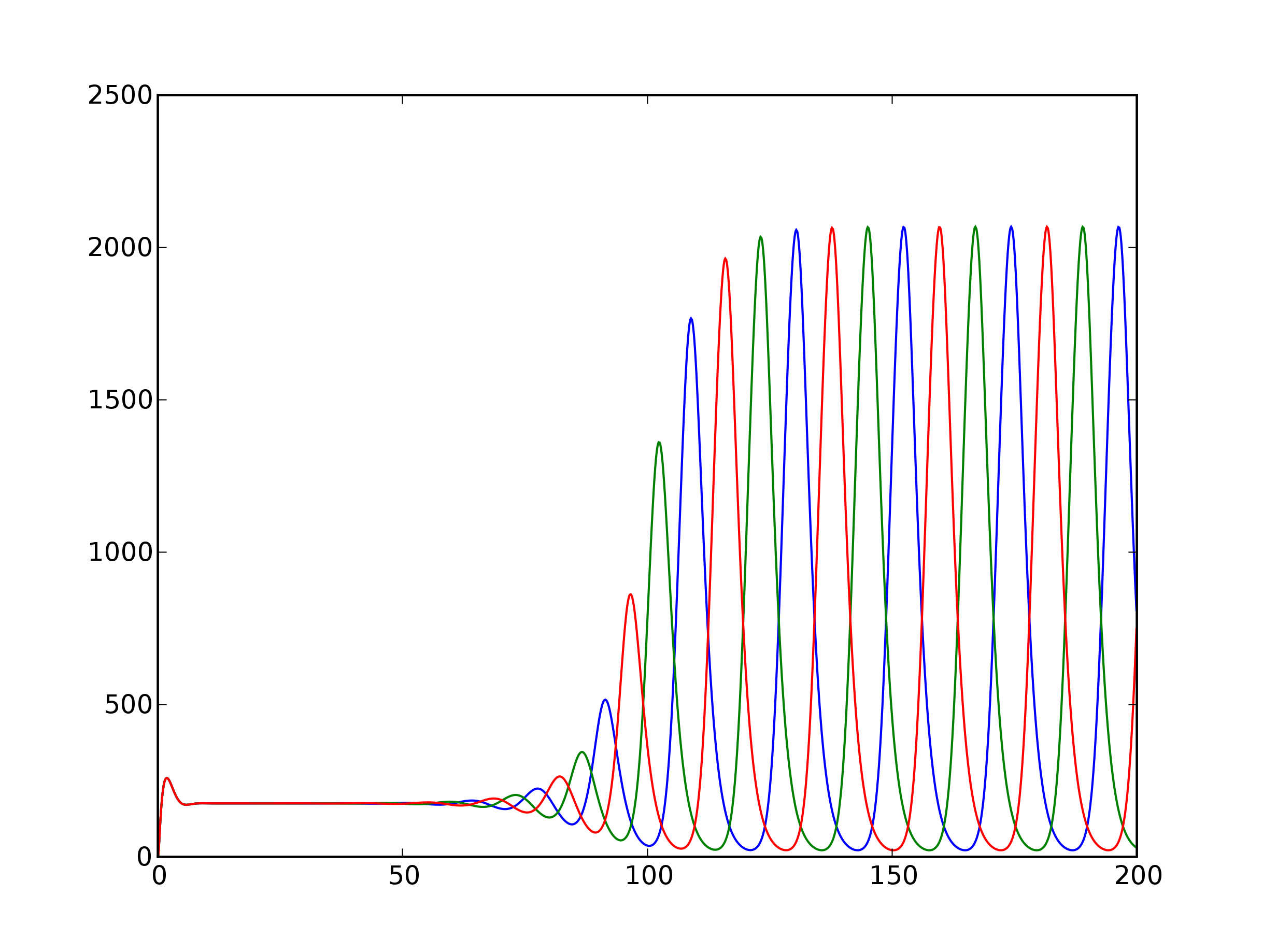
   • Note: The default parameter values given in the __init__ method for alpha, alpha0, and beta are chosen such that the Repressilator should spontaneously oscillate, rather than converge to a steady state. See Fig. 2(b) of the Repressilator paper: the X in parameter space is roughly at alpha=216, beta=5, with alpha0/alpha=0.001, and n=2. (Note that beta as defined on the y-axis of Fig. 2(b) is the inverse of that described on p. 337 of the paper, as lifetimes are proportional to the inverse of decay rates.)
6. Implement the method dydt(y,t,alpha,n,alpha0,beta) that returns the right hand side of the scaled dynamical equations. This will be used with odeint for integrating the dynamics in time. You'll notice in the hints file that this is declared as a staticmethod, which is a way of defining a method without having the self passed as the implicit first parameter to the method. We need to do this since odeint needs a right-hand-side function that takes y0 and t as argument, not an instance of a class. See the Python docs to learn more about staticmethods. (Alternatively, if you're feeling very adventurous, define instead a method make_dydt that returns a function for use with odeint, with the current values of the model parameters alpha, alpha0, and beta hardwired in, rather than passed as args.)
7. Implement the run method. This should integrate the dynamical equations for a specified time interval, and store the trajectory in an instance variable self.traj. Since you might want to call run multiple times in succession, you will want to append the result of the integration to self.traj rather than overwriting it with each function call.
   • NOTE: scipy.append(array1, array2) can be used to append one array to another, but its behavior is different than the append method for Python lists. Whereas the list.append method modifies the list in place (and returns None), the scipy.append method concatenates two arrays and returns the result. (I find this choice unfortunate.)
8. Implement a method plot that will plot the dynamical trajectory of the Repressilator. You might want to include options for showing just the mRNA or protein concentrations, as well as an option for converting back from scaled units to absolute units to compare with Fig. 1(c) of the Repressilator paper.
9. Implement a method find_steady_state to find the steady-state concentrations of mRNAs and proteins, based on the values of the model parameters. This will involve using scipy.optimize.fsolve to find a set of concentrations cstar for which the concentrations do not change in time.
10. The steady state is stable only for certain parameters. Where it is unstable, it gives rise to the oscillations of interest. Fig. 1(b) of the Repressilator paper shows a phase diagram delineating the stable and unstable regimes in parameter space. Write a method plot_phase_boundary that sweeps over parameters alpha, and generates the corresponding values of beta, using fsolve, that delineate the stability boundary. Make a plot of the phase boundary for the parameter values specified in Fig. 1(b).
    • If you're interested in a derivation of this stability result, look at section 19.3.3 of Physical Biology of the Cell
11. Implement a method in_steady_state that returns True if the system is in a steady state, or False if it is not. Compute the instantaneous velocity (i.e., that returned by dydt) and see if its vector norm is small (e.g., below 1.0e-3).
12. For various sets of parameters in the alpha-beta plane, compute whether the Repressilator has a stable steady state. Plot the sets of parameters for which the steady state is stable, and overlay this with a plot of the computed stability boundary.