Background

In this module, you will be exploring the dynamics of the fully-mixed SIR (Susceptible-Infected-Recovered) model, the cornerstone of epidemiological modeling. Specifically, you will build simulations for both deterministic and stochastic versions of the SIR model, in order to explore the onset of large outbreaks at a critical reproductive number, the size of those outbreaks as a function of model parameters, and their distribution within the stochastic model. See these lecture notes for a brief overview of the field and some of the material covered in this module, as well as the review article by Review paper: Rock et al. and the book chapter from Easley and Kleinberg (links also at left).

Procedure

1. Hints file: Download the Python hints file from the link at the left, make a copy of it into an answer version of the file, and load it into your preferred editing environment.
2. Base class: Define a base class called SIRsystem which will store state and parameter information for each of the two SIR models you will subsequently build (deterministic and stochastic).
   • Define an initializer (__init__(self,beta,gamma,S,I,R)) which accepts model parameters beta and gamma, and initial numbers of hosts in each of the S,I and R compartments.
   • Define a method named reset(self,S,I,R,t=0.) which will enable you to reset the SIRsystem to a specified (S,I,R,t) state, and reinitializes the trajectory to this state. This will be useful when running multiple trajectories, sparing you from having to recreate a new SIR system each time.
   • Define a method named get_total_infected(self) which returns the total number of hosts either currently or previously infected.
3. Deterministic SIR: Define a subclass of SIRsystem called DeterministicSIRsystem which will be used for simulating deterministic SIR models.
   • Add a method dydt(self,y,t) which defines the right-hand-side of the equation dy/dt = dydt(y,t) for the SIR model, for use with the scipy.integrate.odeint integrator. (See XXX for information on the syntax for such a function, but note also that because this is defined as a method on the class rather than as a free-standing function, the first argument of the function must be the self instance rather than the current state vector y.)
   • Add a method run(self,T) that integrates the ODE for the deterministic SIR model from time 0. to time T, storing the result in the self.trajectory instance.
4. Deterministic outbreaks (part 1): Generate and plot some trajectories of your DeterministicSIRsystem for various parameter values. Plot the S,I and R trajectories as a function of time. Although the model as written formally depends on two parameters (beta and gamma), the equations of model can be nondimensionalized to show that only their ratio R_0 = beta/gamma is relevant for describing the dynamics of the system. For R_0 < 1, you should observe that outbreaks die out quickly. For R_0 > 1, they grow and eventually die out.
5. Deterministic outbreaks (part 2): Write a function SimulateDeterministicOutbreakSize(N, R0_range) which will simulate deterministic SIR outbreaks in a population of size N hosts, for various values of R0 specified, starting each outbreak from a single infected individual. Run for a long time until the outbreak has died out, and record and return the total size of the outbreak (number of individuals infected over the course of the outbreak).
6. Deterministic outbreaks (part 3): Write a function CalculateDeterministicOutbreakSize(N, R0_range) which will calculate the final size of a deterministic SIR outbreak for the various values of R0 specified, by using scipy.optimize.fsolve to solve the implicit equation for the total number of recovered individuals as $t\to\infty$: $R(infinity) = 1-exp(-R_0 * R(infinity))$. Once you've got this working, calculate and plot the theoretical outbreak size alongside the simulated outbreak sizes from part 2 above as a function of R_0.
7. Stochastic SIR: Define a subclass of SIRsystem called StochasticSIRsystem which will be used for simulating stochastic SIR models.
   • Add a method step(self) which takes one step of the Gillespie algorithm (direct method, as described in the StochasticCells exercise). Return an integer index indicating which transition has fired, and the time at which it fired.
   • Add a method run(self,T,make_traj=True) that runs multiple Gillespie steps to stochastically simulate the system dynamics from time 0 to time T, storing the result in the self.trajectory instance (if make_traj parameter is True) and also storing the reaction times in a separate array self.times.
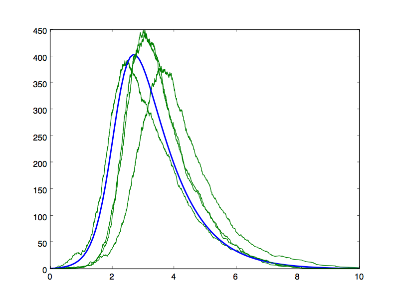
   • Test your stochastic simulator by running and plotting several trajectories for various values of model parameters beta and gamma (or, alternatively, R_0). For the same parameter values, generate deterministic trajectories and plot those alongside the stochastic trajectories. For R_0>1, some trajectories should look like noisy versions of the corresponding deterministic trajectory for the same parameter values, although some trajectories will also die out without generating large outbreaks even though R_0 is supercritical. While the deterministic model might have been defined in terms of concentrations of S,I and R hosts (i.e., fractions of the total population size), the stochastic version should be defined in terms of absolute numbers of hosts in each state, so you may need to rescale one trajectory by a factor of N to make a meaningful comparison.
8. Stochastic outbreaks (part 1): Write a function called StochasticOutbreaksSizeDistribution(N, beta, gamma, Nruns) that generates Nruns different stochastic outbreaks in a population of size N with model parameters beta and gamma. Record and return arrays for both the total size of each outbreak (total number of infected individuals) and the total duration of each outbreak (time required for the outbreak to die out).
9. Stochastic outbreaks (part 2): Using the function you just wrote, generate outbreak size distributions for a range of subcritical and critical values of R_0, i.e., for R_0 <= 1. (Since we are only interested here in measuring final outbreak statistics, rather than dynamical trajectories, you should run this with make_traj=False to avoid wasting time building up trajectories that you will not use.) Plot these outbreak size distributions alongside each other (probability P(n) of observing an outbreak of size n). What do these distributions look like, and how do they change as R_0 approaches 1 from below. At R_0=1, the outbreak size distribution should obey a power-law, indicating the onset of extensive, large outbreaks at criticality. On a log-log plot, this distribution should look roughly like a straight line. Download and install the Python package powerlaw and use it to estimate the scaling exponent for the outbreak size and outbreak duration distributions.
10. Stochastic outbreaks (part 3): Now generate outbreak size distributions for a range of supercritical parameters. As noted before, some stochastic outbreaks die out before being able to generate large numbers of infecteds, even for R_0>1. (This is in contrast to the deterministic model.) For various R_0 larger than 1, generate a large number of outbreaks (e.g., 1000) and record the outbreak size statistics. As R_0 gets larger and larger, the probability of having a "small" outbreak (of size O(1) rather than O(N)) will diminish, since the infection is more likely to spread. Theoretical results state that the probability of small outbreaks will decrease like 1/R_0. Calculate the fraction of small outbreaks as a function of R_0 (using some reasonable threshold to distinguish between small and large outbreaks) and compare with theory.

Notes

---