Background

In this exercise we will explore the dynamics of the double pendulum. This is a classic example of a chaotic system. It will give a rather brief overview of some of the concepts you would see in a nonlinear dynamics class. 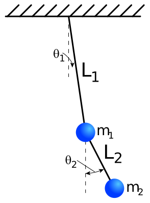The double pendulum, illustrated to the right, is a much richer system than the simple pendulum. The equations of motion involve four variables: theta1,theta2,omega1,omega2. These are derived in several places. For example: MathWorld, Wikipedia, and myphysicslab.

Learning Goals

Science: The double pendulum will illustrate a simple chaotic system. You will learn how to deal with time series data, how to make Poincare sections, and how to diagnose chaos.

Computation: You will learn how to deal with multidimensional data sets in an interactive environment.

Procedure

Setup

1. It is strongly recommended that you first do the Pendulum Exercises. Much of the current exercise will make more sense after understand how to work with that simpler system.
2. This exercise is written assuming you will use odeint as your integrator. Feel free to use smartodeint instead. Some of the exercises (such as making the Poincare section) will then be a little easier. You will however need to write a parametricplotfunction routine, which can be modelled off of plotfunction.
3. Create a new directory
4. Download the following files:
   • Double Pendulum Hints File
5. Rename DoublePendulumHints.py as DoublePendulum.py, and open it in a text editor (for example, kate, gedit, or emacs) or in the ipython notebook dashboard (started with ipython notebook --pylab inline).
6. Move to the correct directory and start Python with ipython --pylab, or click on the notebook in dashboard.
7. The equations of motion for the Double Pendulum are given in the hints file as DoublePendulumDerivArray. This routine is alread filled in so that you don't have to go through the tedium of copying/coding formulas. The math to calculate these derivatives is straightforward -- we urge you to write down the Lagrangian and work out the dynamics, and see if you agree with what we wrote. Note that DoublePendulumDerivArray is called by not only vars and t but also by all of the relevant parameters: (l1,l2,m1,m2,g). There are several methods of sending these parameters to the function. We will use a technique which is common in Python interfaces. In the method used here, every time we call DoublePendulumDerivArray we will include the parameters. This means that the integrator, odeint needs to know about the parameters. This is done through the use of the args argument, which is a tuple which is unpacked and then fed into the derivative function.
   • Note that there are alternative approaches to handling the problem of passing arguments to a function. For example, one can write a constructor which you call to create a function for which the parameters are hard coded. Yet another approach is to pass not a function, but a more sophisticated object which knows about the parameters.
8. Calling odeint with DoublePendulumDerivArray, and dealing with the output can cause headaches. Good programing practice would have you write a wrapper around odeint which takes care of all of these issues.
   • Write a routine called DoublePendulumTrajectory which takes the initial values, the timestep, the number of timesteps, and the parameter, then returns a dictionary. the dictionary should have the following keys: "times", "theta1", "theta2", "omega1", "omega2", "parameters". The values associated with the first five keys are time series. The parameters key stores the parameters as a dictionary. It will be useful to also include in "parameters" a key "energy" which returns the energy of the system at the initial time. We have included a doublependulumenergy function.
     • Test by running this with a small amplitude oscillation, and with l2 and m2 very small, say: trial1=DoublePendulumTrajectory(initial_omega1=0.1,l1=1,l2=0.01,m1=1,m2=0.01,g=1,timestep=0.1,numstep=200). The motion of theta1 will essentially be that of a simple pendulum.
     • Plot a time series with plot(trial1["times"],trial1["theta1"]) or a phase-plane plot with plot(trial1["theta1"],trial1["omega1"])
9. Experiment with the case l1=l2=m1=m2=1. Start with small values of initial_omega1. For example, try the following: traj1= DoublePendulumTrajectory(initial_omega1=0.1,timestep=0.1,numstep=2000). Does the result make sense? Plot everything that might be relevant (eg. all of the state variable against eachother).
   • A useful thing is to look at the Fourier transform of the time series for the angle theta1. Type f1=scipy.fft(traj1["theta1"]) then plot(abs(f1)). You should see four peaks -- this corresponds to two frequencies (and their negatives). This is because you have excited both the in-phase and out of phase modes.
   • To excite just the in-phase mode, do traj2=DoublePendulumTrajectory(initial_omega1=0.1,initialomega2=0.2,timestep=0.1,numstep=2000). Look at its time series and the Fourier transform. Try exciting the out-of-phase mode. [Hint -- linearize the equations of motion to figure out how to do this.]
10. Try larger amplitudes. You may find it useful to type something like triallist=[(s,DoublePendulumTrajectory(initial_omega1=s,timestep=0.1,numstep=2000)) for s in arange(0.1,3,0.1)].
11. Lets make a few more functions which can be used to investigate this system.
    • Make a function, ShowDoublePendulumTrajectory, which you call with this dictionary which will plot the x-y trajectory of the two pendulum bobs. Try it out.
    • Make a function, ShowDoublePendulumTimeSeries, which will plot the x and y time series for the two bobs.
    • Play with these functions.

Poincare Section

1. You have probably found that it is hard to extract too much info from these time series. The basic problem is that this is a multidimensional data set: we have four state variables, plus time. We can however use a technique from nonlinear dynamics to reduce the size of the data set -- this approach is to make a "Poincare Section", a 2-dimensional cut through the phase space of the system. The first thing to note is that we do not actually have a 5D problem.
   • We have time translational invariance: if at any time the four state variables take on any particular value, then the subsequent dynamics are uniquely defined -- it doesn't matter when that value is attained. Thus we can summarize the dynamics by looking at the trajectories in 4D phase space.
   • We have a conservation law: conservation of energy. Thus for any given initial condition the dynamics are constrained to a three dimensional manifold in the 4D phase space. This allow us to eliminate one variable, giving us a 3D problem.
   • We then just need to sample phase space, constraining one of the variables. To do this, write a routine: ShowDoublePendulumPoincare which is called with the dictionary created by DoublePendulumTrajectory. This function should do the following
     • Find the times at which theta1=0 (or a multiple of 2pi), and for which omega1>0. At each of those times, record theta2 and omega2. The Poincare section is a scatter plot of these values.
       • First you should unpack the data. For example, writing theta1=data["theta1"], and parameters=data["parameters"] and l1=parameters["l1"]. This will make the syntax of the rest of the function simpler.
       • You can bracket the times where theta1 changes sign by looking at the product prodlist=theta1[:-1]*theta1[1:] which is the product of theta1 at each subsequent time intervals. If this is negative at any time slice, then theta1 must change sign between that time slice and the next. We could find the index of those time slices with numpy.where(prodlist<0). We actually need to do some thing more sophisticated:
         • We want to find where theta1 crosses 2*pi*n for any integer n with the further constraint that omega1>0. We can do this by making use of the logical & symbol, and by working with numpy.sin(theta1[:-1]) and numpy.sin(theta1[:-1]).
       • Once you have bracketed the times, there are a few trick you could use to find the values of theta2 and omega2. For example, you could use the event detection approach from the pendulum module. A simpler approach is to interpolate. Suppose that s1=sin(theta1) at time slice i and s2=sin(theta1) at time slice i+1, and that one of s1,s2 is positive and the other is negative. Suppose the values of theta2 at these two slices are θ1,θ2. If we assume a linear relation between s and θ then we should have θ=[(s-s1)θ2-(s-s2)θ1]/(s2-s1). In particular the value of θ when s=0 will be θ0=(s2θ1-s1θ2)/(s2-s1). Implement the function lininterp(xvals,yvals) which implements this linear interpolation.
       • Use a list interpretation to create a list of the interpolated theta2's and omega2's.
       • Make a scatter plot
2. Examine the poincare sections for small amplitude motion. For example longtraj1= DoublePendulumTrajectory(initial_omega1=0.1,timestep=0.1,numstep=60000) then ShowDoublePendulumPoincare(longtraj1). How does this compare to the case when you excite only the in-phase mode?
   • These Poincare sections are indicative of regular (periodic or quasiperiodic) motion. Quasiperiodicity occurs when you have multiple incommensurate frequencies in your motion.
3. Examine larger amplitude motion, for example with initial_omega1=1.3. What feature of the Poincare section is different? Note this is still regular motion. Investigate the time series. What aspect of the motion can be associated with the change in the behavior of the Poincare section?
4. Look at even larger amplitude motion, say initial_omega1=1.5. What happens to the Poincare section? This is indicative of Chaos. What does the fourier spectrum of the time series look like?
5. To see what the Poincare sections should look like, see Introduction to Pendulum Module.

Sensitive dependance on initial conditions

1. Explore how sensitive the trajectories of the pendulum are to small changes in initial conditions. Compare the case where the motion is regular to that of the chaotic regime.

Animation

1. Download the file AnimateDoublePendulum.py. This animation was put together by Bruce Sherwood at North Carolina State. It is covered by a Creative Commons Attribution 2.5 License which essentially means you can use it as you like -- but should properly cite the source. For a list of some of Bruce's other demos (and those of his collaborators), see Public Programs VI and Public Programs VII. Many of these are good examples of making interactive graphics, where you can use the mouse to manipulate things. Note: you need to have "visual" installed to use these.
2. Start a new python session -- do not use the -pylab flag. Type %run AnimateDoublePendulum.py. Watch the behavior. Play with the different parameters -- the lengths of the various bars, the initial conditions, etc.
3. Use this animation to visualize the various different behaviors you saw previously.

Useful Constructions/Syntax

Science Concepts

• Chaos
  • Sensitivity to initial conditions
• Poincare Section
• Phase plane portrait