Background
In this exercise we will explore the dynamics of the simple pendulum. The dynamics of a pendulum is described by an ordinary differntial equation. Solving differential equations on the computer is one of the most common scientific tasks. To solve these equations you approximate the continuous-time evolution with a discrete time step. A good algorithm will be accurate, stable, and produce high fidelity results. We will use the following techniques
- First order methods which we explicitly code:
- The forward Euler method: easy to understand and easy to implement. Tends to be unstable for simple systems, with energy growing in time.
- The symplectic Euler method. Equally easy to implement, plus it has a number of useful properties. The dynamics correspond to an exact solution (up to rounding errors) of an approximate Hamiltonian: it retains volume in phase space, and exactly conserves an approximation to the energy.
- The backward Euler method. This one tends to be very stable, but introduces an artificial damping to the dynamics.
- Sophisticated packages for adaptively solving differential equations. These switch between different orders and between explicit and implicit methods, and are appropriate for most small systems of ordinary differential equations. We will use one of these from scipy.
Learning Goals
Science: You will learn about different algorithms for solving ordinary differential equations in the context of a simple nonlinear dynamical system.
Computation: You will learn to manipulate functions as objects -- passing them as arguments to an ODE integrator. You will learn how to run an interactive python session where one produces and analyzes graphs.Procedure
A forward Euler Integrator for the simple pendulum
- Create a new directory
- Download the following files:
- Read the description of integration strategies: Integration Strategies
- Rename PendulumODEHints.py as PendulumODE.py, and open it in a text editor (for example, kate, gedit, or emacs) or load it into the ipython dashboard (started with ipython notebook --pylab inline) You can leave out the inline flag if you do not want the graphs to appear in the notebook, but rather in a separate window. In this file you will notice Python code that has already been written, but it mostly consists of hints to help you flesh out the code, i.e., comments (lines that begin with #) and documentation strings (material enclosed in triple quotes """ that document what each module, class, and function is about and can be queried with the Python help() function). You will also notice the keyword pass embedded within each function body: pass is a legal Python expression that means "do nothing". The first thing you will do when you start to define a function is to remove the pass statement and replace it with new code.
- If you are using the terminal interface than open a terminal window, move to the correct directory and start ipython with the following command ipython -pylab, otherwise click on the file in the ipython dashboard. The "flag" pylab automatically imports the functions from the pylab module into the main namespace, and sets up the graphics software for an interactive session.
- Test that pylab has correctly loaded. If you are in a terminal, or if you started the notebook without the inline flag then:
- Type figure(1) and then plot([0,1,2,1,2]). You should see a graph appearing.
- Next try plot([0.1,0.2,0.3,0.4,4],[0,1,2,1,2]). Another line should appear on your plot.
- Start a second figure by typing figure(2). Fill it with a graph by typing another plot command. Have fun.
- If you have used the inline flag, then instead type the two plot commands in one cell. Hit shift-enter to run them. You should see both lines appearing on the graph.
- Edit the PendulumODE.py file, creating the function EulerIntegratePendulum (using natural units).
- If you are in a terminal, type %run PendulumODE.py to load in the function you just defined. If you are in a notebook, just hit "shift-enter" on the cell.
- Test by exploring small amplitude oscillations through the following procedure
- Generate some data by typing testtrajectory=EulerIntegratePendulum(InitialTheta=0.1,InitialOmega=0,InitialTime=0,FinalTime=16*pi,dt=4*pi/1000).
- Plot a time series by typing figure(3) then plot(testtrajectory[0],testtrajectory[1]). Plot angular frequency on this same graph with plot(testtrajectory[0],testtrajectory[2]). Go to the pylab tutorial to learn how to label figures. Note that you do not have to type the show() commands that are listed in the tutorial -- this is because we are in "interactive mode". Label the axes (using commands xlabel and ylabel), the plot (using title) and the two curves (using legend).
- Plot the trajectory in phase space by typing figure(4) then plot(testtrajectory[1],testtrajectory[2]). Label the axes.
- Test how your algorithm responds to making the stepsize larger by typing testtrajectory2=EulerIntegratePendulum(InitialTheta=0.1,InitialOmega=0,InitialTime=0,FinalTime=16*pi,dt=4*pi/100). Plot the trajectories on the same graphs. IE. type figure(3) then plot(testtrajectory2[0],testtrajectory2[1]).
- How does this compare? Play a bit.
- Complete the PendulumEnergy function.
- If you are in a terminal type %run PendulumODE.py to load this function. In a notebook instead hit shift-enter.
- You can use this function to get how the energy evolves by typing elist=map(PendulumEnergy,testtrajectory[1],testtrajectory[2]) and elist2=map(PendulumEnergy,testtrajectory2[1],testtrajectory2[2]). [Alternatively, you can forgo the map command if you pass in array objects. For example, elist=PendulumEnergy(array(testtrajectory[1]),array(testtrajectory[2])). It turns out that the array handling routines are faster than the mapping routines, so this is actually the prefered approach.] How does this energy behave when your timestep is large? Plot them on another graph (say figure 5). This energy non-conservation is what motivates using a symplectic algorithm.
- Play with your integrator. Can you, for example, produce a phase plane portrait where you plot a number of trajectories with different initial conditions?
A Symplectic Integrator for the simple pendulum
- Implement the symplectic Euler method (see Integration Strategies ) -- the routine SymplecticIntegratePendulum should only differ from EulerIntegratePendulum in a couple lines.
- Compare with your forward Euler integrator. In particular, what happens to the energy over time when the timestep is large?
A backward Euler Integrator for the simple pendulum
- Implement the backward Euler algorithm (see Integration Strategies ). For this you will have to solve a transcendental
equation at each step. We will use the scipy.optimize.fsolve function to solve this equation.
- For more information of fsolve, have a quick look at NanoPy 5
- To save writing, in the PendulumODE.py file we define fsolve=scipy.optimize.fsolve which makes a function in the main namespace which is the same as scipy.optimize.fsolve.
- The equations that we need to solve to find the new theta and omega depend on the
old parameters and the timestep. We need a mechanism to set these when we call fsolve. There are several
strategies for this -- the one we will use is to take advantage of the third argument to fsolve.
As examples of how to do this, see the four findsqrt routines w
in the Hints file. These are examples of using fsolve to
calculate square roots (of course the built in sqrt command is better).
- Of particular note, the first routine, findsqrt uses the following construction: fsolve(sqrtfun,estimate,(num)). What this does is it repeatedly calls sqrtfun(guess,num) until sqrtfun(guess,num)=0. An even more sophisticated example of this is findnthroot, which has a line fsolve(nthrootfun,estimate,(num,n)). This repeatedly calls nthrootfun(guess,num,n) until nthrootfun(guess,num,n)=0.
- Use whichever paradigm you prefer. The hints file assumes you are using the paradigm of the function findsqrt. In this approach we get the new theta and omega at each time step by performing a function call that looks something like newthetaomegalist=fsolve(BackwardPendulumFunction,(oldtheta,oldomega),((oldtheta,oldomega),dt)). The function BackwardPendulumFunction is described in the hints file. If using this approach, complete that function, and complete BackwardIntegratePendulum.
- How does the backward Euler integrator compare to the other two algorithms? Note, this nicely demonstrates that implicity methods (such as the backward Euler) are more stable. [Things do not tend to run off to infinity.] On the other hand, the decay in the energy that you see is non-physical.
A general Euler Integrator
We now want to explore some variants of the pendulum. We could write more special-purpose routines for applying these various algorithms to different sets of dynamical equations, but we would then be reproducing a lot of code. Here comes a dramatic leap: we abstract the details of the specific system in a function, and then we can write a function that takes the system-specific function as an argument. The function that we call with will encode the differential equation. The function fsolve that we used in the previous exerciese used this same strategy. We are going to choose the syntax for our function so that it matches that of scipy's built in ODE solver. We will just use the forward Euler algorithm since it is the simplest to implement. When we really want well controlled results we will use odeint.
Our integrator will be called with the following syntax: EulerIntegrate(DerivitiveArrayFunc,InitialValues,times).
- DerivitiveArrayFunc will be a function of two variables: a list/tuple/array of dynamical variables, and time. DerivitiveArrayFunc will return a list/tuple/array, which represents the derivative of the dynamical variables evaluated at the given time.
- InitialValues will be the inital values of the dymanical variables.
- times will be a list of the times at which we want the values of the dynamical variables. For this function we will do a single step of the forward Euler algorithm to go from one time to the next. Although this syntax is the same as for odeint, the odeint function will actually break each of these time segments into small pieces in a dynamic way so as to provide a sufficiently accurate solution to the differential equation.
- Write the routine EulerIntegrate.
- Test by directly comparing the results to the output of EulerIntegratePendulum. To do this it will be convenient to write a function PendulumDerivArray. When called with a tuple vars=(x,v) and the time t, this function will return the tuple (dx/dt,dv/dt).
- Your EulerIntegrate function should give identical results to EulerIntegratePendulum. Run with a small number of timesteps to compare explicitly.
Using ODEInt
- You probably want to bring odeint into the main namespace. To do this type from scipy.integrate import *. After that you can call odeint instead of scipy.integrate.odeint. In an interactive session this will save you a lot of typing.
- Have a quick look at NanoPy 5
- If you want to see what is happening under the hood, you can have a look at the reference for the underlying Fortran rountines, odepack.
- odeint is called with the same syntax as EulerIntegrate. The t argument functions a little differently though. As with EulerIntegrate, the integrator returns the function evaluated at those times. Unlike EulerIntegrate however, the odeint integrator uses an addaptive step size. At the end it interpolates through this addaptive grid to evaluate the functions at the times you specified. From a design point of view this is probably not ideal. This choice was made because it gives a syntax which is similar to what is used by MatLab. [see section on an improved odeint interface for one way to add functionality.]
- Verify that odeint correctly gives the dynamics of the pendulum.
The Period of the Pendulum (optional)
Here we will look at two ways to calculate the period of the pendulum. First the elementary way which involves a simple definite integral. Second using a method called
For the first part, recall that because the pendulum is described by an autonomous differential equation (meaning that the right hand side has no explicit time dependance). One can use the chain rule:
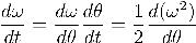 Since
Since
 we get energy conservation
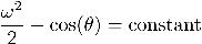 This is integrated to get that the period of a pendulum swinging with maximum amplitude
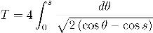
- Write the function PendulumPeriod which takes s as its argument and returns the period of the pendulum. It should use the scipy.integrate.quad function.
- For very small angles, this function should return numbers very close to 2 pi. For angles approaching Pi, the period should become large.
- Make a function PlotPeriod which plots the period of a pendulum as a function of angle.
Next we will do the same thing using a more generic approach that will work even when there is no energy conservation. Starting from our initial conditions (with theta>0 and omega=0) we will integrate the differential equation forward in time by a small amount. If theta is still positive, we keep repeating until theta changes sign. We thereby bracket the time at which the pendulum has travelled a quarter period.
To find the exact quarter period, we use the following trick. We change independent variables from time to angle, writing
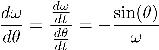 and
and
 then integrating these equations from the point that our last integration ended to the point where
theta=0.
then integrating these equations from the point that our last integration ended to the point where
theta=0.
- The first step is to write a function which when called by vars=(omega,t) and theta returns a tuple (domega/dtheta,dt/dtheta). We will call this function PendulumDOmegaTDTheta.
- Next write the function ODEPendulumPeriod, which given the initial angle will return the period. It will use the algorithm described above, and repeated in the hints file.
- Compare the results to PendulumPeriod
Animation
There are several techniques for animating the dynamics of a pendulum. One example is shown in PendulumAnimation.py or PendulumAnimation.enthought.py. The former is for users of "visual", while the latter is for users of "Enthought python". Enthought users should start ipython with the "-pylab" flag if they want to interact with the animation.This program uses the symplectic Euler algorithm to update the animation. Try it out. Play with parameters. What happens if you switch from the symplectic Euler algorithm to the forward Euler algorithm (this just requires switching the order of two lines of code).
Note, design-wise PendulumAnimation.py is essentially a procedural program -- much like you would write in Basic. A more sophisticated example is in the Walker Exercise. Note, there is nothing wrong with a procedural program. There is no need to make something "object oriented" or "functional" just for the sake of using a structured programing paradigm.
An Improved interface to odeint (optional)
One important aspect of the interactive mode of scientific programming is that you want the interface with the functions/classes to be intuitive. The idea is that instead of spending your mental effort trying to remember a bunch of archane syntax, you should be able to focus on the science. Here is what I want from a numerical integrator:
- It should take as input the differential equations, the initial conditions, the interval over which I want the solution, and the desired accuracy of the solution.
- It should give as output an object that represents the solution to the equation. This object should be capable of giving me the value of the function at any time that I request. I should not need to give it a list of time values before solving the equation.
pendtheta1,pendomega1=smartodeint(PendulumDerivArray,(2,0),(0,25))
rt=pendtheta1.roots()
rt[:-1]-rt[1:]
You have to agree that this is a lot more satisfactory that the approach we used above.[You would plot the trajectory with plotfunction(pendtheta1)].
Another integrator (optional)
- You may want to play with the object oriented integrator scipy.integrate.ode. Look at the help documentation and see what you can do.
Useful Constructions/Syntax
- Trigonometric functions: numpy.sin, numpy.cos. These are also in pylab and in scipy.
- Numpy/Scipy arrays.
- scipy.integrate.odeint
- pylab.figure
- pylab.scatter
- pylab.plot
- map
- scipy.integrate.fsolve
- *args and **args
- from MODULE import FUNCTIONS as NAME
- scipy.integrate.quad
- list comprehensions
- numpy.arange
- raise
- hasattr
- scipy.interpolate.UnivariateSpline
- scipy.transpose
- scipy.integrate.ode
Science Concepts
Notes
Units in computation
Units are important. For example, errors in units leads to Airline Crashes, Medical Errors, and lost satellites. They also are a problem for computation. Most programing environments (python included) work with pure dimensionless numbers. It is not easy to propegate units around. An obvious strategy is that you pick some standard units which you will measure all quantities in: for example meters, seconds, and kg.
This strategy has some problems. Consider, for example, the pendulum. If we measure time in seconds, then we will need to know g, L, and M before we can write down the differential equation (or at least the relevant combination of these), and we will need to pass this quantity around in our program. We then will have to adjust all of our parameters whenever we change things. We run the risk of findin very small numbers, or very large numbers. [For example if we were dealing with a nano-Pendulum, then the oscillations might only take a million'th of a second.] A more robust approach is to write your program using natural units. In the pendulum example, dimensional analysis says that the only relevant timescale must by sqrt(g/L). It therefore makes sense to use that for our unit of time.
Such crazy units work great for the computer program. Automatically interesting things tend to happen on the scale of natural units. How do you, as a scientist, keep track of what units you are using? The easiest thing is to write a function to which you pass all of the physical parameters. It will spit back what the time unit is in physical quantities.
Some researchers prefer to just include a comment in the file which expresses what the units are. That can work too, but the advantage of making a function that calculates the units is that you can use that routine internally to do conversions.
Strategies for working in an interactive environment
- Don't reuse the same name over and over. If you run the integrator with 10 different parameters, give each of those 10 a new name. That way you can replot the data at a later time in the session.
- If you don't want to forget what parameter a particular name is associated with, copy and paste the line that generated it into a text file. This makes a nice record of your session.
- If you find yourself doing something tedious, then stop and reevaluate how you are doing it. For example, suppose you want to run your Euler integrator with 10 different timesteps, and then plot a graph of the time series. Don't do this by hand. Add a function to your PendulumODE.py file which does it for you. At first you can hard code it for the parameters you want. If you find you are doing that task a lot with different parameters, then make the function take the parameters as an argument. Programs are organic -- they grow as you need more funcitonality.
Lambda Functions
By now you should be comfortable with the idea that a function is an object that can be passed from one place to another. For simple functions, the syntax for doing this can become a little awkward. For example, suppose you wanted to integrate the ODE for a decaying exponential. You might type some thing like this:
def oscfunc(x,t):
	return -x
ser1=odeint(oscfunc,1,arange(0,10,0.1))
It turns out that there is a shorthand notation for defining functions. The following code is equivalent to the last one:
oscfunc=lambda x,t:-x
ser1=odeint(oscfunc,1,arange(0,10,0.1))
The keyword "lambda" is used to define a function. The syntax above defines a function of two variables, which returns the negative of the first argument. Where this notation becomes usefull is when you omit the function definition in the first place, and just type
ser1=odeint(lambda x,t:-x,1,arange(0,10,0.1))The equivalent command for a pendulum would be
pendser=odeint(lambda x,t:(x[1],-sin(x[0])),(1,0),arange(0,10,0.1))In a program it is probably best to avoid lambda functions. The construction using def is much more readable. On the other hand, in an interactive session the savings on typing can be significant.